In some scientific contexts it is natural to regard time as discrete. This is the case in digital electronics, in parts of economics and finance theory, also in impulsively driven mechanical systems. Evidently, discrete variables should be used in modelling animal populations where successive generations do not overlap.

Let us consider discrete time systems. In a general case the system has the form

If the function is linear with respect to then one has a linear system. Thus in the one dimensional case the linear discrete system can be written as

and being given constants.

The graph of the linear function is a straight line. If the line does not go through the origin of coordinates then the function is called affine.

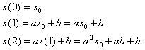
Let us work out the first few values:

For one has

provided and

when If then and regardless of the value of If then and

In the two or more dimensional case the discrete linear dynamical system can be written as

where and are vectors and stands for a matrix.

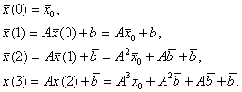
Similarily to the previous case one can compute the iterations etc. to obtain

In the general case we have

which can be simplified to

provided is invertible.

If the absolute values of the eigenvalues of are less than 1 (hence is invertible), then tends to zero matrix. Hence

Alternatively, if some eigenvalues have absolute value bigger than 1, then blows up, and for most we have

There are, ofcourse, exceptional values of For example, if 1 is not an eigenvalue of and

then

for all

Finally, if some eigenvalues have absolute value equal to 1 and the other eigenvalues have absolute value less than 1, we see a range of behaviour. The system might stay near or it might blow up.

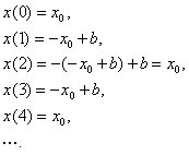
Consider now the case

First, if then (in the one dimensional case). So, if then Otherwise is stuck at regardless of the value of

Second, if then we observe that

Thus we see that oscillates between two values, and But if i.e. then is stuck at the fixed point