This course is about how to predict the future from a knowledge of how things are at the present time together with a set of rules governing the changes that will occur. These changes are often modelled by differential equations.
Some common examples of differential equation models are
Once the differential equations have been determined the goal is then to use them to predict future behaviour. There are three main approaches for making these predictions
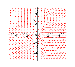
A first mental picture of what the solutions look like can be obtained
from the direction field. This is a plot of the gradient at specific
points. An example of a direction field diagram is shown below. The arrows
point in the direction of increasing t.

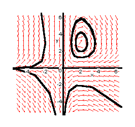
The next step is to sketch a number of trajectories in the x-y plane.
This gives the phase plane or phase portrait for the system.
The aim is to sketch enough of the solutions so that the general qualitative
behaviour of all solutions can be surmised by looking at the picture. A
number of initial points are chosen scattered over the x-y plane and the
solution curve through each of the initial points is sketched. Exactly
which initial points and how many are needed to make a good phase plane
diagram requires trial and error and some artistic feeling. Here is an
example of a phase portrait.

The final step is to interpret the phase portrait.
Look at the point A and trace the trajectory through A following the direction of the arrows. The trajectory is a closed curve and you will eventually return to A. This sort of trajectory represents cyclic motion.
Now trace the trajectory through the point B. In this case the trajectory
starts with large negative x and small positive y. At first
x and y both increase until x reaches a maximum value.
Then x decreases while y continues to increase until as ![]() x becomes large and negative and y becomes large and positive.
x becomes large and negative and y becomes large and positive.
This implies that the starting point is crucial as the trajectories can exhibit different behaviour for different initial conditions.
Next look at the trajectories starting at C and D. You should find that these are straight line trajectories. In this case C moves towards the origin whereas D moves away from it. A straight line trajectory is called a directrix and is an asymptote for the system.
Look at the remaining trajectories and try to describe what happens
as ![]() . Look
carefully at the direction of the arrows. Fill your answers in the space
provided in the handbook.
. Look
carefully at the direction of the arrows. Fill your answers in the space
provided in the handbook.
By clicking on (0,0) and
(2,3)
you can see an enlarged sections of the graph .Look closely at the phase
portrait in the region of the points ![]() .
What do you think would happen to a point which starts at
.
What do you think would happen to a point which starts at ![]() or
or ![]() ?
Would it move away from the initial point or would it stay there for all
time? Such points are called equilibrium points.
?
Would it move away from the initial point or would it stay there for all
time? Such points are called equilibrium points.
Look again at the region close to the point ![]() .
Look carefully at the direction of the arrows in the region of
.
Look carefully at the direction of the arrows in the region of ![]() .
Do they point towards
.
Do they point towards ![]() or
away from it? Imagine a point slightly displaced from
or
away from it? Imagine a point slightly displaced from ![]() .
Would it return to
.
Would it return to ![]() or
move further away from it? Is the point
or
move further away from it? Is the point ![]() stable
or unstable?
stable
or unstable?
Now look at the direction of the arrows in the region of the point ![]() .
The arrows are neither pointing towards nor away from the point
.
The arrows are neither pointing towards nor away from the point ![]() but
are forming closed curves around the point. Such a point is said to be
neutrally stable.
but
are forming closed curves around the point. Such a point is said to be
neutrally stable.
The phase plane is just one way of visualising the solutions of differential
equations. Not all the information about a particular solution can be seen
by a glance at the phase portrait. We do not see the time variable, so
we do not see how fast the solution traverses the curve. This can be seen
by giving the x-t and y-t graphs along with the phase portrait.
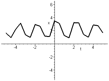
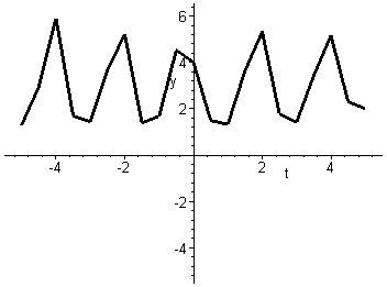
These are commonly referred to as time series plots. Some time series plots
are shown below.


These two graphs show x and y against t for the
trajectory passing through the point ![]() .
They confirm oscillatory motion for this trajectory with period approximately
equal to two seconds..
.
They confirm oscillatory motion for this trajectory with period approximately
equal to two seconds..
This investigation suggests that equilibrium points, asymptotes and stability are three important features in the interpretation of a phase diagram. In this unit you will learn