CASE STUDY
The following example will show how a variety of these methods can be used
![]() Worked example
Worked example
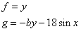
The motion of an unforced pendulum subject to viscous damping is modelled by the second order differential equation
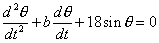
where b, is a constant

and

Substituting
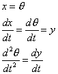
into the original equation gives
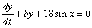
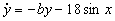
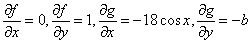
Thus the equations become

The first step in analysing a nonlinear system is to find the equilibrium points.
These occur when

Therefore, y=0 and sinx =0
The equilibrium points are ![]()
The second step is to classify the equilibrium points of the linearisations by examining the Jacobian matrices.
Let
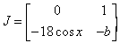
Then
and the Jacobian matrix of the linearisations is given by
If n is odd

Tr = -b and det = -18
and the equilibrium point of the linearisation is a saddle. By the linearisation theorem the nonlinear system shows similar behaviour close to the equilibrium points and they are therefore unstable and nonlinear saddles.
If n is even
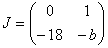
Tr = -b and det = 18
The behaviour of the equilibrium point of the linearisation depends on the value of b. If
![]() the equilibrium
point is stable
the equilibrium
point is stable
![]() the equilibrium
point is unstable
the equilibrium
point is unstable
![]() the equilibrium
point is a centre
the equilibrium
point is a centre
By the linearisation theorem the equilibrium points of the nonlinear system are
stable if ![]()
unstable if ![]()
If b=0 the system needs further investigation.
Further investigation
To investigate further look for a conserved quantity. This can be done by finding a first integral.
Since b=0 the equations for the system become

Dividing gives
![]()
![]()
![]()
Since this function exists for all values of (x,y) it follows that
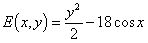
is a conserved quantity.
Next we need to see if the equilibria are local maxima or minima of E(x,y)


The equilibria occur at ![]() with n even therefore
with n even therefore

and

Thus the equilibria are stationary points of E(x,y)
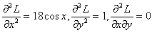
Next find the Hessian matrix
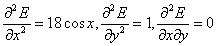
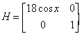
Therefore
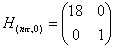
The eigenvalues are 18 and 1 and so the equilibrium point is a maximum
Thus the level curves of E(x,y) are closed curves surrounding the equilibrium points and since it is a conserved system the solutions of the system lie along these curves. Thus the solution curves also form closed curves around the equilibrium points and they are nonlinear centres and neutrally stable.
Thus the equilibrium points are all unstable if b<0
alternately an unstable nonlinear saddle and a stable equilibrium point if b>0
alternately an unstable nonlinear saddle and a nonlinear centre if b=0
Draw phase portraits for appropriate values of b to confirm this analysis.
Proving the existence of a centre using reversibility
An alternative method of proving the existence of a centre when b=0
would be to prove the system reversible. Try this method for yourselves.
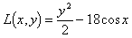
An alternative approach to this problem is to use the Lyapunov function
1) first we need to prove it is a Lyapunov function
![]()
![]()
![]()
provided b![]()
If b=0 then L(x,y) is a conserved quantity ,if b>0 L(x,y) is a Lyapunov function
2)To describe the behaviour of a system we first need to find the equilibrium points given by

therefore the equilibrium points occur at ![]()
We need to find if these are stationary points of L(x,y)
At the point ![]()


Therefore the equilibria are stationary points of L(x,y)
We now need to determine whether they are maxima or minima of L(x,y)
Therefore the Hessian matrix is given by
If n is odd
the Hessian matrix is given by
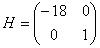
The eigenvalues are of opposite signs and the equilibrium point is therefore a saddle of L(x,y). Thus if b>0 the solution curves of the nonlinear system cross the curves of L(x,y) and the equilibria are nonlinear saddles and unstable.
If n is even

The eigenvalues are both negative and the equilibrium point is a minimum of L(x,y). The level curves of L(x,y)=C therefore form closed curves surrounding the equilibria. If b>0 the solutions of the nonlinear system cross the curves of L(x,y) and the equilibria are therefore attractors and stable.
If b=0 L(x,y) is a conserved quantity and the system is conservative. Thus the solution curves of the system must follow the level curves of L(x,y) and will form closed curves surrounding the equilibria. Thus the equilibria are nonlinear centres and neutrally stable.