In this section you will

investigate the geometric behaviour of nonlinear systems and their linearisations close to their equilibrium points.

learn under what conditions a nonlinear system behaves locally like its linearisation

learn how to classify the equilibrium points
 

2.2.1     Linearisation Theorem
The idea of linearisation is to use a linear system to approximate the behaviour of solutions of a nonlinear system near an equilibrium point We are going to investigate the equilibrium points of the linearisation and see what, if anything, we can deduce about the equilibrium points of the nonlinear system. Can we deduce the stability of their equilibrium points? Can we say anything about the geometric behaviour of solutions close to the equilibrium points?

Consider the nonlinear system

with equilibrium point (p,q).

We have already seen that the system may be approximated in the neighbourhood of the equilibrium point by the linear system

Where J is the Jacobian matrix

Look at the tr- det diagram for linear systems. The boundary lines for stability are trace=0 and det=0. Since linearisation is an approximation it is when the trace and determinant of the Jacobian matrix lie on the boundary lines between stability and non-stability and the system is, therefore, very sensitive to small changes that there are likely to be differences in the long term behaviour of a nonlinear system and its linearisation. You already know that if det=0 the linear system is non simple and without further investigation nothing can be deduced about the behaviour of the system close to an equilibrium point. Likewise a nonlinear system is not a simple system if its linearisation is non simple and we are, therefore, unable to classify its equilibrium points from its linearisation. The stability under the condition trace=0 needs careful investigation.

Investigation 1

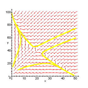
Consider again the competing species model

with equilibrium points (0,0), (0,100), (50,0) and (20,40)

Here is its phase plane diagram.

For each equilibrium point you are going to plot the phase diagram of the nonlinear system close to the equilibrium point and compare it with  the phase diagram of its linearisation. You can open a maple window  which will contain the appropriate programs by clicking in turn on the equilibrium points (0,0) ,  (50,0) , (20,40) , (0,100) .

Do the linearisations show the same geometric behaviour as the nonlinear system  close to an equilibrium point?

This investigation suggests that the behaviour of a nonlinear system close to an equilibrium point mimics the behaviour of its linearisation. The extent to which this is true is summarised in the following important theorem, proofs of which were published independently by the American mathematician Philip Hartman (1964) and the Soviet mathematician David Grobman (1965).

2.2.2     Hartman Grobman Theorem
If the linearisation matrix J has no zero or purely imaginary eigenvalues, then the phase portrait for the nonlinear system near an equilibrium point is similar to the phase portrait of its linearisation.

worked example 1

2.2.3     Limitations of the Hartman Grobman Theorem
    Note that the Hartman-Grobman theorem has two serious limitations. First it tells us nothing when the linearisation is non simple or a centre. Secondly, when the theorem does apply it provides information only about the behaviour of solutions near the equilibria. In order to make global predictions we need more information. These limitations will be illustrated in the following examples.

Investigation 2

To investigate solutions of a nonlinear system when the linearisation is a centre.

You are going to plot the phase diagrams of the nonlinear system  close to its equilibrium point and also the phase diagram of its linearisation. You can open the Maple window by clicking on  Investigation2

Investigation3

To look at the global phase portrait of a nonlinear system.

You are going to plot the phase diagrams of the nonlinear system both close to the equilibrium point and also over a wider range of values of x and y. You can open the Maple window by clicking on  Investigation 3
 

2.2.4     Summary

1. If the linearisation is a stable node or stable focus the equilibrium point of the nonlinear system is an attractor and stable.
2. If the linearisation is an unstable node or unstable focus the equilibrium point of the nonlinear system is a repeller and unstable
3. If the linearisation shows a saddle then the nonlinear system is a nonlinear saddle and is unstable
4. If the linearisation shows a centre it is not yet possible to determine the nature of the equilibrium point of the nonlinear system.
5. If the linearisation is a non simple system the nonlinear system is also classed as non simple and we are unable to classify the system from its linearisation.